Writing reproducible reports in R with markdown, knitr and pandoc
So you have some code, data and a cool result, now it’s time to communicate this with your collaborators (or supervisor). What do you do? In this guide, we want to show you how to write nice, reproducible reports using some of the fantastic, free tools and packages that are now on offer. These tools will help you communicate your science, and hopefully mean that you never copy and paste your R output again.
As a start, let’s review the key components to any good analysis:
- Data
- Code used to analyse the data
- Figures and tables generated by the code
- Text, interpreting the figures and results, and describing the methods.
These elements come together in the form of a report. As scientists, we write many reports, both small and large. Large reports like papers, are rare, but we write smaller reports all the time. These include all the preliminary results, weekly updates, emails with figures, and simply one’s own note taking, written during the lifespan of a project. Traditionally, most biologists do stages 2 and 3 in R, then fire up Word or Powerpoint and copy-paste everything for stage 4. That works, but there several downsides to this approach:
- lots of time wasted, plus copy and pasting sucks
- your interpretation is separated from your code
- Word doesn’t offer syntax highlighting, so it’s hard to read code presented this way,
- Word documents can’t be tracked (very well) under version control
- the report cannot be regenerated without doing it all that copying and pasting over again.
Thankfully, there now exists a much nicer way to write reports, using the wonderful package knitr, a simple text-markup language called markdown, and the universal document conversion program called pandoc. It’s also now possible to weave your interpretation (stage 4) in with your R code (stage 2) and results (stage 3), to produce nice, self-contained and reproducible reports. Together, these provide a powerful tool set for scientists looking to save time and do reproducible research.
What is markdown and why use it?
The start of this process is the markdown language. Markdown’s goal is to be “as easy-to-read and easy-to-write as is feasible”. In practice, it is a simple set of formatting commands applied to a plain text document that can be easily converted into fancy formatted html, pdf or word docs. But unlike html, rtf, latex, or pretty much any other markup text, markdown is very readable, as is. And because it uses Plain text, the files are small and easy to edit on a variety of devices.
As scientists we write a lot, not just papers, but also notes, code, emails, reminders, to do lists, blog posts etc. Increasingly, I use markdown for most of my note taking and report writing.
Lots of people have written talking about how wonderful markdown is, e.g. here, and here.
Why you will fall in love with Markdown - http://t.co/PGsCPe5s
— Chen Luo (@chenluois) October 14, 2012
Because it is plain text, you can write markdown in any program, all you need is a syntax guide. However, the best test editors also allow you to view your code as formatted html. I use Sublimetext on my computer, and notesy on my iphone. Here’s a list of 78 other editors to checkout.
Oh yeah, mark down docs usually end with extension .md, or .markdown.
RMarkdown
Markdown proved so useful that many different coding groups adopted it, but also adding there own ‘flavours’. So far we know of the following:
- the original markdown
- github flavoured markdown,
- pandoc markdown, and
- multimarkdown.
Each of these offers a slightly different set of features.
RStudio implements something called “R-flavoured markdown” (or RMarkdown) which can be based on any of these flavours. In addition, it includes “code blocks” – pieces of code that will be run by R. These look like this:
```{r}
mean(1:10) # or some other code
```
which produces something like this:
```
mean(1:10) # or some other code
```
```
## [1] 5.5
```
which would be rendered by Markdown like this:
1
| |
1
| |
R markdown is used within Rstudio and allows R code to be weaved in
with bits of text. Files written in R markdown have the extension
.Rmd.
Think of R markdown as something that compiles into one of the above markdown variants. But first, you need to run all the bits of R code
Reports with knitr
The knitr package was written to combine elements of RMarkdown and R code within a single document. The best way to realise the strength of knitr is to start with an example.
Open up Rstudio and install the knitr package
1
| |
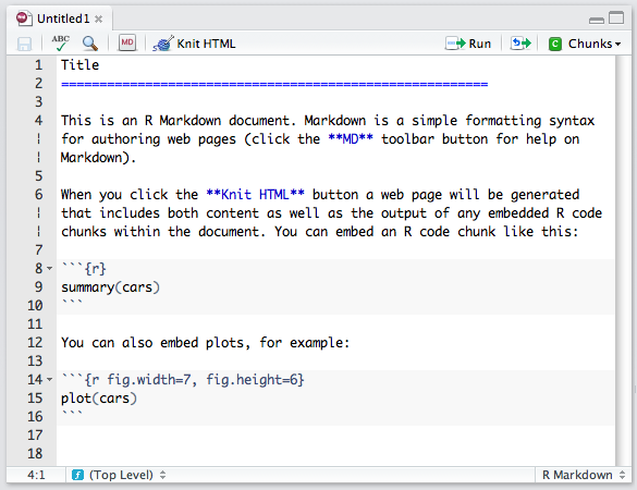
Then open this demo file and click the knit HTML button
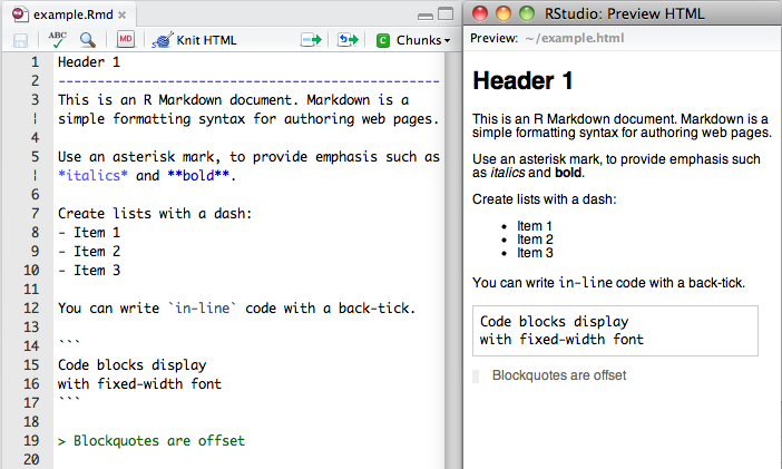
This file is written in RMarkdown and includes bits of text and code. The code bits are the “chunks” surrounded tick marks.
 .
.
Clicking on knit HTML does several things
- It runs all the bits of code in the file
- It generates a markdown file, including bits of the original document and it’s output.
- It converts the markdown document into html.
You can also make the document from the console, with the following set of commands:
1 2 3 4 | |
Note, for this code to work, the example file needs to be in your working directory, or you need to provide the path to the RMD file:
1
| |
OK, so you have a document (html file), where you can document your analyses. Now just replace the example code with some real material and away you go.
Some benefits of this approach include:
- no copying and pasting
- your report can be easily updated, once you have more data, new ideas etc
- because they are just like any other code, you can track your knitr scripts under version control.
- if it is important, you can show bits of the code used to generate the results.
- your analysis is fully transparent and reproducible.
People now use knitr for all sorts of things, e.g.
- writing reports of their data (here’s one by Rich as Rmd and html )
- preparing tutorials
- writing blog posts.
I love #knitr for #rstats with @rstudioapp! Made my first report yesterday, now generating customised reports for >50 data contributors.
— Daniel Falster (@adaptive_plant) April 18, 2013
Tricks to working with knitr and Rstudio
For beginners, the following resources may prove useful
- Rstduio includes a markdown syntax guide, just click the MD button in the toolbar
- Also see their online documentation on using Rmarkdown (http://www.rstudio.com/ide/docs/authoring/using_markdown)
Avoiding trouble
We have advised you
previously
against using setwd() in your scripts. That is even more important
here. Changing the working directory within an Rmd file will lead to
trouble. Therefore we advise you to write all Rmd files to run
assuming they are in the root directory of your project.
Revealing and hiding code and output
You can choose what gets included in the evnetual report, by setting options for each code chunk.
echo= TRUE: choose this if you want the code to be displayed in the report, ofFALSEif you want to hide it.results= "hide": choose this if you want ot hide the results of running the code.eval =FALSE: causes the current chunk not to be evaluated.
For more detail about these options, checkout
- RStduio’s guide on Customizing Chunk Options
- the worked example in our example script
- full documentation on the knitr site.
Converting to different document formats
Now what if you want to produce another document type, instead of an html file? Enter pandoc.
Pandoc – love it! Cross platform command-line converter to/from HTML, Markdown, docx, EPUB, LaTeX, DocBook, etc. http://t.co/OAtPTt9T
— Sam Dutton (@sw12) December 4, 2012
According to it’s creator, “If you need to convert files from one markup format into another, pandoc is your swiss-army knife. It can read a variety of inputs, including markdown, reStructuredText, HTML, LaTeX, MediaWiki markup, and DocBook XML; and it can write plain text, markdown, reStructuredText, XHTML, HTML 5, LaTeX (including beamer slide shows), ConTeXt, RTF, DocBook XML, OpenDocument XML, ODT, Word docx, GNU Texinfo, MediaWiki markup, EPUB, FictionBook2, Textile, groff man pages, Emacs Org-Mode, AsciiDoc, and Slidy, Slideous, DZSlides, or S5 HTML slide shows. It can also produce PDF output on systems where LaTeX is installed.””
First, you’ll need to download and install pandoc. Once installed you can then use the pnadoc function, included with the knitr package to convert the generated md file into whatever format you like. E.g. to convert our example above into a word doc, we write:
1 2 3 4 | |
Here comes the future: presentations and everything
In addition to writing reports, you can also use knitr and Rmarkdown to write slide shows directly from within Rstudio, the publish these straight to the Rpubs website. To use the presentation function, you need to download and install the development version of Rstudio, but this feature will no doubt become standard in the near future.
For example, here’s a presentation on R resources, by Scott Chamberlain.
Reproducible research
So there you have it, a set of tools for doing reproducible research in R. In our view, markdown needs a little more work before we’d recommend it for writing an entire paper, but it’s fantastic for most of the preliminary work. And it’s especially good for doing reproducible research, when combined with version control and some nice R code.
More information
Here’s another knitr example script by Jeromy Anglim.
Also, keep an eye out for Yihui Xie’s upcoming book:
Dynamic Documents with R and knitr (Chapman & Hall/CRC The R Series) by Yihui Xie http://t.co/31VZrxjW9r via @amazon
— Flávio Clésio (@flavioclesio) June 21, 2013