The usual way of plotting to a file is to open a plotting device (such as pdf or png) run a series of commands that generate plotting output, and then close the device with dev.off(). However, the way that most plots are developed is purely interactively. So you start with:

1
2
3
4
5
6
7
8
9

set.seed(10)
x <- runif(100)
y <- rnorm(100, x)
par(mar=c(4.1, 4.1, .5, .5))
plot(y ~ x, las=1)
fit <- lm(y ~ x)
abline(fit, col="red")
legend("topleft", c("Data", "Trend"),
       pch=c(1, NA), lty=c(NA, 1), col=c("black", "red"), bty="n")

Then to convert this into a figure for publication we copy and paste this between the device commands:

1
2
3

pdf("my-plot.pdf", width=6, height=4)
  # ...pasted commands from before
dev.off()

This leads to bits of code that often look like this:

1
2
3
4
5
6
7
8
9
10
11

# pdf("my-plot.pdf", width=6, height=4) # uncomment to make plot
set.seed(10)
x <- runif(100)
y <- rnorm(100, x)
par(mar=c(4.1, 4.1, .5, .5))
plot(y ~ x, las=1)
fit <- lm(y ~ x)
abline(fit, col="red")
legend("topleft", c("Data", "Trend"),
       pch=c(1, NA), lty=c(NA, 1), col=c("black", "red"), bty="n")
# dev.off() # uncomment to make plot

which is all pretty ugly. On top of that, we’re often making a bunch of variables that are global but are really only useful in the context of the figure (in this case the fit object that contains the trend line). An arguably worse solution would be simply to duplicate the plotting bits of code.

A partial solution:

The solution that I usually use is to make a function that generates the figure.

1
2
3
4
5
6
7
8
9
10
11

fig.trend <- function() {
  set.seed(10)
  x <- runif(100)
  y <- rnorm(100, x)
  par(mar=c(4.1, 4.1, .5, .5))
  plot(y ~ x, las=1)
  fit <- lm(y ~ x)
  abline(fit, col="red")
  legend("topleft", c("Data", "Trend"),
         pch=c(1, NA), lty=c(NA, 1), col=c("black", "red"), bty="n")
}

Then you can easily see the figure

1

fig.trend() # generates figure

or

1
2

source("R/figures.R") # refresh file that defines fig.trend
fig.trend()

and you can easily generate plots:

1
2
3

pdf("figs/trend.pdf", width=6, height=8)
fig.trend()
dev.off()

However, this still gets a bit unweildly when you have a large number of figures to make (especially for talks where you might make 20 or 30 figures).

1
2
3
4
5
6
7

pdf("figs/trend.pdf", width=6, height=4)
fig.trend()
dev.off()

pdf("figs/other.pdf", width=6, height=4)
fig.other()
dev.off()

A full solution

The solution I use here is a little function called to.pdf:

1
2
3
4
5
6
7

to.pdf <- function(expr, filename, ..., verbose=TRUE) {
  if ( verbose )
    cat(sprintf("Creating %s\n", filename))
  pdf(filename, ...)
  on.exit(dev.off())
  eval.parent(substitute(expr))
}

Which can be used like so:

1
2

to.pdf(fig.trend(), "figs/trend.pdf", width=6, height=4)
to.pdf(fig.other(), "figs/other.pdf", width=6, height=4)

A couple of nice things about this approach:

• It becomes much easier to read and compare the parameters to the plotting device (width, height, etc).
• We’re reduced things from 6 repetitive lines to 2 that capture our intent better.
• The to.pdf function demands that you put the code for your figure in a function.
• Using functions, rather than statements in the global environment, discourages dependency on global variables. This in turn helps identify reusable chunks of code.
• Arguments are all passed to pdf via ..., so we don’t need to duplicate pdf’s argument list in our function.
• The on.exit call ensures that the device is always closed, even if the figure function fails.

For talks, I often build up figures piece-by-piece. This can be done like so (for a two-part figure)

1
2
3
4
5
6
7
8
9
10
11
12
13

fig.progressive <- function(with.trend=FALSE) {
  set.seed(10)
  x <- runif(100)
  y <- rnorm(100, x)
  par(mar=c(4.1, 4.1, .5, .5))
  plot(y ~ x, las=1)
  if ( with.trend ) {
    fit <- lm(y ~ x)
    abline(fit, col="red")
    legend("topleft", c("Data", "Trend"),
           pch=c(1, NA), lty=c(NA, 1), col=c("black", "red"), bty="n")
  }
}

Now – if run with as

1

fig.progressive(FALSE)

just the data are plotted, and if run as

1

fig.progressive(TRUE)

the trend line and legend are included. Then with the to.pdf function, we can do:

1
2

to.pdf(fig.progressive(TRUE),  "figs/progressive-1.pdf", width=6, height=4)
to.pdf(fig.progressive(FALSE), "figs/progressive-2.pdf", width=6, height=4)

which will generate the two figures.

The general idea can be expanded to more devices:

1
2
3
4
5
6
7

to.dev <- function(expr, dev, filename, ..., verbose=TRUE) {
  if ( verbose )
    cat(sprintf("Creating %s\n", filename))
  dev(filename, ...)
  on.exit(dev.off())
  eval.parent(substitute(expr))
}

where we would do:

1
2

to.dev(fig.progressive(TRUE),  pdf, "figs/progressive-1.pdf", width=6, height=4)
to.dev(fig.progressive(FALSE), pdf, "figs/progressive-2.pdf", width=6, height=4)

Note that with this to.dev function we can rewrite the to.pdf function more compactly:

1
2

to.pdf <- function(expr, filename, ...)
  to.dev(expr, pdf, filename, ...)

Or write a similar function for the png device:

1
2

to.png_function(expr, filename, ...)
  to.dev(expr, png, filename)

(As an alternative, the dev.copy2pdf function can be useful for copying the current contents of an interactive plotting window to a pdf).

In many analyses, data is read from a file, but must be modified before it can be used. For example you may want to add a new column of data, or do a “find” and “replace” on a site, treatment or species name. There are 3 ways one might add such information. The first involves editing the original data frame – although you should never do this, I suspect this method is quite common. A second – and widely used – approach for adding information is to modify the values using code in your script. The third – and nicest – way of adding information is to use a lookup table.

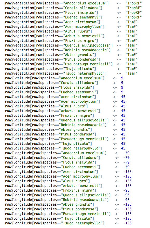
One of the most common things we see in the code of researchers working with data are long slabs of code modifying a data frame based on some logical tests.Such code might correct, for example, a species name:

1
2

raw$species[raw$id=="1"] <- "Banksia oblongifolia"
raw$species[raw$id=="2"] <- "Banksia ericifolia"

or add some details to the data set, such as location, latitude, longitude and mean annual precipitation:

1
2
3
4
5

raw$location[raw$id=="1"] <-"NSW"
raw$latitude[raw$id=="1"] <- -37
raw$longitude[raw$id=="1"] <- 40
raw$map[raw$id=="1"] <- 1208
raw$map[raw$id=="1"] <- 1226

In large analyses, this type of code may go for hundreds of lines.

Now before we go on, let me say that this approach to adding data is much better than editing your datafile directly, for the following two reasons:

1. It maintains the integrity of your raw data file
2. You can see where the new value came from (it was added in a script), and modify it later if needed.

There is also nothing wrong with adding data this way. However, it is what we would consider messy code, for these reasons:

• Long chunks of code modifying data is inherently difficult to read.
• There’s a lot of typing involved, so lot’s of work, and thus opportunities for error.
• It’s harder to change variable names when they are embedded in code all over the place.

A far nicer way to add data to an existing data frame is to use a lookup table. Here is an example of such a table, achieving similar (but not identical) modifications to the code above:

1

read.csv("dataNew.csv")

##   lookupVariable lookupValue newVariable              newValue
## 1             id           1     species  Banksia oblongifolia
## 2             id           2     species    Banksia ericifolia
## 3             id           3     species       Banksia serrata
## 4             id           4     species       Banksia grandis
## 5                         NA      family            Proteaceae
## 6                         NA    location                   NSW
## 7             id           4    location                    WA
##            source
## 1  Daniel Falster
## 2  Daniel Falster
## 3  Daniel Falster
## 4  Daniel Falster
## 5  Daniel Falster
## 6  Daniel Falster
## 7  Daniel Falster

The columns of this table are

• lookupVariable is the name of the variable in the parent data we want to match against. If left blank, change all rows.
• lookupValue is the value of lookupVariable to match against
• newVariable is the variable to be changed
• newValue is the value of newVariable for matched rows
• source includes any notes about where the data came from (e.g., who made the change)

So the table documents the changes we want to make to our dataframe. The function addNewData.R takes the file name for this table as an argument and applies it to the data frame. For example let’s assume we have a data frame called data

myData

##          x     y id
## 1  0.93160 5.433  1
## 2  0.24875 3.868  2
## 3  0.92273 5.944  2
## 4  0.85384 5.541  2
## 5  0.30378 3.985  2
## 6  0.41205 4.415  2
## 7  0.35158 4.440  2
## 8  0.13920 3.007  2
## 9  0.16579 2.976  2
## 10 0.66290 5.315  3
## 11 0.25720 3.755  3
## 12 0.88086 5.345  3
## 13 0.11784 3.183  3
## 14 0.01423 3.749  4
## 15 0.23359 4.264  4
## 16 0.33614 4.433  4
## 17 0.52122 4.393  4
## 18 0.11616 3.603  4
## 19 0.90871 6.379  4
## 20 0.75664 5.838  4

and want to apply the table given above, we simply write

1
2
3

source("addNewData.r")
allowedVars <- c("species", "family", "location")
addNewData("dataNew.csv", myData, allowedVars)

##          x     y id              species     family location
## 1  0.93160 5.433  1 Banksia oblongifolia Proteaceae      NSW
## 2  0.24875 3.868  2   Banksia ericifolia Proteaceae      NSW
## 3  0.92273 5.944  2   Banksia ericifolia Proteaceae      NSW
## 4  0.85384 5.541  2   Banksia ericifolia Proteaceae      NSW
## 5  0.30378 3.985  2   Banksia ericifolia Proteaceae      NSW
## 6  0.41205 4.415  2   Banksia ericifolia Proteaceae      NSW
## 7  0.35158 4.440  2   Banksia ericifolia Proteaceae      NSW
## 8  0.13920 3.007  2   Banksia ericifolia Proteaceae      NSW
## 9  0.16579 2.976  2   Banksia ericifolia Proteaceae      NSW
## 10 0.66290 5.315  3      Banksia serrata Proteaceae      NSW
## 11 0.25720 3.755  3      Banksia serrata Proteaceae      NSW
## 12 0.88086 5.345  3      Banksia serrata Proteaceae      NSW
## 13 0.11784 3.183  3      Banksia serrata Proteaceae      NSW
## 14 0.01423 3.749  4      Banksia grandis Proteaceae       WA
## 15 0.23359 4.264  4      Banksia grandis Proteaceae       WA
## 16 0.33614 4.433  4      Banksia grandis Proteaceae       WA
## 17 0.52122 4.393  4      Banksia grandis Proteaceae       WA
## 18 0.11616 3.603  4      Banksia grandis Proteaceae       WA
## 19 0.90871 6.379  4      Banksia grandis Proteaceae       WA
## 20 0.75664 5.838  4      Banksia grandis Proteaceae       WA

The large block of code is now reduced to a single line that clearly expresses what we want to achieve. Moreover, the new values (data) are stored as a table of data in a file, which is preferable to having data mixed in with our code.

You can use this approach You can find the example files used here, as a github gist.

Acknowledgements: Many thanks to Rich FitzJohn and Diego Barneche for valuable discussions.

Until recently, I hadn’t given much attention to organising files in my project. All the documents and files from my current project were spread out in two different folders, with very little sub folder division. All the files where together in the same place and I had multiple versions of the same file, with different dates. As you can see, things were getting a bit out of control.

Following advice from by Rich and Daniel, I decided to spend a little time getting organised, adopting a directory layout with the following folders:

• Data: which contains both my base (raw) data and the processed data
• Output: data and figures generated in R
• R: R scripts with all new functions I created as part of the cleaning directory process and in an attempt to write nicer code.
• Analysis (R file): R script sourcing all the functions necessary for the analysis

At the same time I started using version control with git. As a result, I no longer need to create a new file every time I make a change, and each of the files in the analysis directory is unique.

Setting up the new directory and sorting the existing files in the new folders didn’t take long and was relatively easy. Now it is really simple to find files and keep track of current and old figures. I no longer need to use spotlight to find the latest version of each script. From my experience this improved the organization and efficiency of my project; I highly recommend keeping a good project layout.

R allows a lot of “computation on the language”, simply meaning that we can look inside objects easily. Here is a function that returns the number of lines in a function.

1
2
3
4
5

function.length <- function(f) {
  if (is.character(f))
    f <- match.fun(f)
  length(deparse(f))
}

This works because deparse converts an object back into text (that could in turn be parsed):

1

writeLines(deparse(function.length))

1
2
3
4
5
6

function (f) 
{
    if (is.character(f)) 
        f <- match.fun(f)
    length(deparse(f))
}

so the function.length function is itself 6 lines long by this measure. Note that the formatting is actually a bit different, in particular indentation, braces position and spacing is different, following the likes of the R-core style guide.

Most packages consist mostly of functions: here is a function that extracts all functions from a package:

1
2
3
4
5
6
7

package.functions <- function(package) {
  pkg <- sprintf("package:%s", package)
  object.names <- ls(name=pkg)
  objects <- lapply(object.names, get, pkg)
  names(objects) <- object.names
  objects[sapply(objects, is.function)]
}

Finally, we can get the lengths of all functions in a package:

1
2

package.function.lengths <- function(package)
  vapply(package.functions(package), function.length, integer(1))

Looking at the recommended package “boot”

1
2

library(boot)
package.function.lengths("boot")

1
2
3
4
5
6
7
8
9
10
11
12
13
14
15
16
17
18

     abc.ci            boot      boot.array         boot.ci 
         54             126              56              80 
   censboot         control            corr            cum3 
        137              72               8               8 
     cv.glm     EEF.profile      EL.profile          empinf 
         42              16              27              79 
   envelope        exp.tilt      freq.array        glm.diag 
         56              49               7              19 
 glm.diag.plots     imp.moments        imp.prob    imp.quantile 
         69              37              34              39 
imp.weights       inv.logit jack.after.boot       k3.linear 
         34               2              69              14 
     lik.CI   linear.approx           logit     nested.corr 
         36              34               2              28 
    norm.ci          saddle    saddle.distn         simplex 
         33             179             281              65 
   smooth.f       tilt.boot          tsboot      var.linear 
         36              57              97              14 

I have 138 packages installed on my computer (mostly through dependencies – small compared with the ~4000 on CRAN!). We need to load them all before we can access the functions within:

1
2
3
4

library(utils)
packages <- rownames(installed.packages())
for (p in packages)
  library(p, character.only=TRUE)

Then we can apply the package.function.lengths to each package.

1

lens <- lapply(packages, package.function.lengths)

The median function length is only 12 lines (and remember that includes things like the function arguments)!

1

median(unlist(lens))

1

[1] 12

The distribution of function lengths is strongly right skewed, with most functions being very short. Ignoring the 1% of functions that are longer than 200 lines long, the distribution of function lengths looks like this:

1
2

tmp <- unlist(lens)
hist(tmp[tmp <= 200], main="", xlab="Function length (lines)")

Then plot the distribution of the per-package median (that is, for each package compute the median function length in terms of lines of code and plot the distribution of those medians).

1
2

lens.median <- sapply(lens, median)
hist(lens.median, main="", xlab="Per-package median function length")

The median package has a median function length of 16 lines. There are handful of extremely long functions in most packages; over all packages, the median “longest function” is 120 lines.

This issue plagues at least Excel 2008 and 2011, and possibly other versions.

Basically, saving a file as comma separated values (csv) uses a carriage return \r rather than a line feed \n as a newline. Way back before OS X, this was actually the correct Mac file ending, but after the move to be more unix-y, the correct line ending should be \n.

Given that nothing has used this as the proper line endings for over a decade, this is a bug. It’s a real pity that Microsoft does not see fit to fix it.

Why this is a problem

This breaks a number of scripts that require specific line endings.

This also causes problems when version controlling your data. In particular, tools like git diff basically stop working as they work line-by-line and see only one long line (e.g. here). Not having diff work properly makes it really hard to see where changes have occurred in your data.

Git has really nice facilities for translating between different line endings – in particular between Windows and Unix/(new) Mac endings. However, they do basically nothing with old-style Mac endings because no sane application should create them. See here, for example.

A solution

There are at leat two stack overflow questions that deal with this (1 and (2).

The solution is to edit .git/config (within your repository) to add lines saying:

1
2
3

[filter "cr"]
    clean = LC_CTYPE=C awk '{printf(\"%s\\n\", $0)}' | LC_CTYPE=C tr '\\r' '\\n'
    smudge = tr '\\n' '\\r'

and then create a file .gitattributes that contains the line

1

*.csv filter=cr

This translates the line endings on import and back again on export (so you never change your working file). Things like git diff use the “clean” version, and so magically start working again.

While the .gitattributes file can be (and should be) put under version control, the .git/config file needs to be set up separately on every clone. There are good reasons for this (see here. It would be possible to automate this to some degree with the --config argument to git clone, but that’s still basically manual.

Issues

This seems to generally work, but twice in use large numbers of files have been marked as changed when the filter got out-of-sync. We never worked out what caused this, but one possible culprit seems to be Dropbox (but you probably should not keep repositories on dropbox anyway).

Alternative solutions

The nice thing about the clean/smudge solution is that it leaves files in the working directory unmodified. An alternative approach would be to set up a pre-commit-hook that ran csv files through a similar filter. This will modify the contents of the working directory (and may require reloading the files in Excel) but from that point on the file will have proper line endings.

More manually, if files are saved as “Windows comma separated (.csv)” you will get windows-style line endings (\r\n) which are at least treated properly by git and are in common usage this century. However, this requires more remembering and makes saving csv files from Excel even more tricky than normal.

To re-emphasise our closing message – start using it on a project, start thinking about what you want to track, and start thinking about what constitutes a logical commit. Once you get into a rhythm it will seem much easier. Bring your questions along to the class in 2 weeks time.

Also, to re-emphasise that git is not a backup system. Make sure that you have your work backed up, just in case something terrible happens. I recommend crash plan which you can use for free for backing up onto external hard drives (and for a fee).

Feedback

We welcome any and all feedback on the material and how we present it. You can give anonymous feedback by emailing G2G admin (you should have the address already – I’m only not putting it up here in a vain effort to slow down spam bots). Alternatively, you are welcome to email either or both of us, or leave a comment on a relevant page.

Writing code is fast becoming a key - if not the most important - skill for doing research in the 21st century. As scientists, we live in extraordinary times. The amount of data (information) available to us is increasing exponentially, allowing for rapid advances in our understanding of the world around us. The amount of information contained in a standard scientific paper also seems to be on the rise. Researchers therefore need to be able to handle ever larger amounts of data to ask novel questions and get papers published. Yet, the standard tools used by many biologists - point and click programs for manipulating data, doing stats and making plots - do not allow us to scale-up our analyses to match data availability, at least not without many, many more ‘clicks’.

Why writing code saves you time with repetitive tasks, by Bruno Oliveira

The solution is to write scripts in programs like R, python or matlab. Scripting allows you to automate analyses, and therefore scale-up without a big increase in effort.

Writing code also offers other benefits to research. When your analyses are documented in a script, it is easier to pick up a project and start working on it again. You have a record of what you did and why. Chunks of code can also be reused in new projects, saving vast amount of time. Writing code also allows for effective collaboration with people from all over the world. For all these reasons, many researchers are now learning how to write code.

Yet, most researchers have no or limited formal training in computer science, and thus struggle to write nice code (Merali 2010). Most of us are self-taught, having used a mix of books, advice from other amateur coders, internet posts, and lots of trial and error. Soon after have we written our first R script, our hard drives explode with large bodies of barely readable code that we only half understand, that also happens to be full of bugs and is generally difficult to use. Not surprisingly, many researchers find writing code to be a relatively painful process, involving lots of trial and error and, inevitably, frustration.

If this sounds familiar to you, don’t worry, you are not alone. There are many great R resources available, but most show you how to do some fancy trick, e.g. run some complicated statistical test or make a fancy plot. Few people - outside of computer science departments - spend time discussing the qualities of nice code and teaching you good coding habits. Certainly no one is teaching you these skills in your standard biology research department.

Learn to code! I worry that most biologists leave uni lacking #1 skill for 21st cent biology. For inspiration code.org #CODE

— Daniel Falster (@adaptive_plant) February 27, 2013

Observing how colleagues were struggling with their code, we (Rich FitzJohn and Daniel Falster) have teamed up to bring you the nice R code course and blog. We are targeting researchers who are already using R and want to take their coding to the next level. Our goal is to help you write nicer code.

By ‘nicer’ we mean code that is easy to read, easy to write, runs fast, gives reliable results, is easy to reuse in new projects, and is easy to share with collaborators.

We will be focussing on elements of workflow, good coding habits and some tricks, that will help transform your code from messy to nice.

The inspiration for nice R code came in part from attending a boot camp run by Greg Wilson from the software carpentry team. These boot camps aim to help researchers be more productive by teaching them basic computing skills. Unlike other software courses we had attended, the focus in the boot camps was on good programming habits and design. As biologists, we saw a need for more material focussed on R, the language that has come to dominate biological research. We are not experts, but have more experience than many biologists. Hence the nice R code blog.

@phylorich Being able to code (in any language) is most important skill for current biology. R is good choice: widely used, high level, free

— Daniel Falster (@adaptive_plant) March 15, 2013

Key elements of nice R code

We will now briefly consider some of the key principles of writing nice code.

Nice code is easy to read

Programs should be written for people to read, and only incidentally for
machines to execute.

Readability is by far the most important guiding principle for writing nicer code. Anyone (especially you) should be able to pick up any of your projects, understand what the code does and how to run it. Most code written for research purposes is not easy to read.

In our opinion, there are no fixed rules for what nice code should look like. There is just a single test: is it easy to read? To check how nice your code is, pass it to a collaborator, or pick up some code you haven’t used for over a year. Do they (you) understand it?

Below are some general guidelines for making your code more readable. We will explore each of these in more detail here on the blog:

• Use a sensible directory structure for organising project related materials.
• Abstract your code into many small functions with helpful descriptive names
• Use comments, design features, and meaningful variable or function names to capture the intent of your code, i.e. describe what it is meant to do
• Use version control. Of the many reasons for using version control, one is that it archives older versions of your code, permitting you to ruthlessly yet safely delete old files. This helps reduce clutter and improves readability.
• Apply a consistent style, such as that described in the
• google R style guide.

Nice code is reliable, i.e. bug free

Occma’s raz0r: if your program isn’t working, it’s probably just a typo in the code, not an undiscovered bug or thing you’re doing wrong

— Alison Abreu-Garcia (@alisonag) April 11, 2013

The computer does exactly what you tell it to. If there is a problem in your code, it’s most likely you put it there. How certain are you that your code is error free? More than once I have reached a state of near panic, looking over my code to ensure it is bug free before submitting a final version of a paper for publication. What if I got it wrong?

It is almost impossible to ensure code is bug free, but one can adopt healthy habits that minimise the chance of this occurring:

• Don’t repeat yourself. The less you type, the fewer chances there are for mistakes
• Use test scripts, to compare your code against known cases
• Avoid using global variables, the attach function and other nasties where ownership of data cannot be ensured
• Use version control so that you see what has changed, and easily trace mistakes
• Wherever possible, open your code and project up for review, either by colleagues, during review process, or in repositories such as github.
• The more readable your code is, the less likely it is to contain errors.

“Every bug is two bugs: the bug in your code, and the test you didn’t write”@estherbester #pycon

— Ned Batchelder (@nedbat) March 15, 2013

Nice code runs quickly and is therefore a pleasure to use

The faster you can make the plot, the more fun you will have.

Code that is slow to run is less fun to use. By slow I mean anything that takes more than a few seconds to run, so impedes analysis. Speed is particularly an issue for people analysing large datasets, or running complex simulations, where code may run for many hours, days, or weeks.

Some effective strategies for making code run faster:

• Abstract your code into functions, so that you can compare different versions
• Use code profiling to identify the main computational bottlenecks and improve them
• Think carefully about algorithm design
• Understand why some operations are intrinsically slower than others, e.g. why a for loop is slower than using lapply
• Use multiple processors to increase computing power, either in your own machine or by running your code on a cluster.

The benefits of writing nicer code

There are many benefits of writing nicer code:

• Better science: nice code allows you to handle bigger data sets and has less bugs.
• More fun: spend less time wrestling with R, and more time working with data.
• Become more efficient: Nice code is reusable, sharable, and quicker to run.
• Future employment: You should consider anything you write (open or closed) to be a potential advert to a future employer. Code has impact. Code sharing sites like github now make resumes for you, to capture your impact. Scientists with an analytical bent are often sought-after in the natural sciences.

If you need further motivation, consider this advice

An advisory pop-up for MS Visual C++

This might seem extreme, until you realise that the maniac serial killer is you, and you definitely know where you live.

At some point, you will return to nearly every piece of code you wrote and need to understand it afresh. If it is messy code, you will spend a lot of time going over it to understand what you did, possibly a week, month, year or decade ago. Although you are unlikely get so frustrated as to seek bloody revenge on your former self, you might come close.

The single biggest reason you should write nice code is so that your future
self can understand it.

As a by product, code that is easy to read is also easy to reuse in new projects and share with colleagues, including as online supplementary material. Increasingly, journals are requiring code be submitted as part of the review process and these are often published online. Alas, much of the current crop of code is difficult to read. At best, having messy code may reduce the impact of your paper. But you might also get rejected because the reviewer couldn’t understand your code. At worst, some people have had to retract high profile work because of bugs in their code.

It’s time to write some nice R code.

For further inspiration, you may like to check out Greg Wilson’s great article “Best Practices for Scientific Computing.”

Acknowledgments: Many thanks to Greg Wilson, Karthik Ram, Scott Chameberlain and Carl Boettiger and Rich FitzJohn for inspirational chats, code and work.

Managing your projects in a reproducible fashion doesn’t just make your science reproducible, it makes your life easier.

— Vince Buffalo (@vsbuffalo) April 15, 2013

Directory layout

A good project layout helps ensure the

• Integrity of data
• Portability of the project
• Easier to pick the project back up after a break

There is no one way to lay a project out. Daniel and I both have different approaches for different projects, reflecting the history of the project, who else is collaborating on that project.

Here are a couple of different ideas for laying a project out. This is the basic structure that I tend to use:

1
2
3
4
5
6

proj/
├── R/
├── data/
├── doc/
├── figs/
└── output/

• The R directory contains various files with function definitions (but only function definitions - no code that actually runs).

• The data directory contains data used in the analysis. This is treated as read only; in paricular the R files are never allowed to write to the files in here. Depending on the project, these might be csv files, a database, and the directory itself may have subdirectories.

• The doc directory contains the paper. I work in LaTeX which is nice because it can pick up figures directly made by R. Markdown can do the same and is starting to get traction among biologists. With Word you’ll have to paste them in yourself as the figures update.

• The figs directory contains the figures. This directory only contains generated files; that is, I should always be able to delete the contents and regenerate them.

• The output directory contains simuation output, processed datasets, logs, or other processed things.

In this set up, I usually have the R script files that do things in the project root:

1
2
3
4
5
6
7

proj/
├── R/
├── data/
├── doc/
├── figs/
├── output/
└── analysis.R

For very simple projects, you might drop the R directory, perhaps replacing it with a single file analysis-functions.R which you source.

The top of the analysis file usually looks something like

1
2
3
4

library(some_package)
library(some_other_package)
source("R/functions.R")
source("R/utilities.R")

…followed by the code that loads the data, cleans it up, runs the analysis and generates the figures.

Other people have other ideas

• Carl Boettiger is an open science advocate who has described his layout in detail. This layout uses R packages for most of the code organisation, and would be a nice approach for large projects.

• This article in PLOS Computational Biology describes a general framework.

Treat data as read only

In my mind, this is probably the most important goal of setting up a project. Data are typically time consuming and/or expensive to collect. Working with them interactively (e.g., in Excel) where they can be modified means you are never sure of where the data came from, or how they have been modified. My suggestion is to put your data into the data directory and treat it as read only. Within your scripts you might generate derived data sets either temporarily (in an R session only) or semi-permanantly (as an file in output/), but the original data is always left in an untouched state.

Treat generated output as disposable

In this approach, files in directories figs/ and output/ are all generated by the scripts. A nice thing about this approach is that if the filenames of generated files change (e.g, changing from phylogeny.pdf to mammal-phylogeny.pdf) files with the old names may still stick around, but because they’re in this directory you know you can always delete them. Before submitting a paper, I will go through and delete all the generated files and rerun the analysis to make sure that I can create all the analyses and figures from the data.

Separate function definition and application

When your project is new and shiny, the script file usually contains many lines of directly executated code. As it matures, reusable chunks get pulled into their own functions. The actual analysis scripts then become relatively short, and use the functions defined in scripts in R. Those scripts do nothing but define functions so that they can always be source()‘d by the analysis scripts.

Setting up a project in RStudio

This gets rid of the #1 problem with most people’s projects face; where do you find the data. Two solutions people generally come up with are:

1. Hard code the full filename for each file you load (e.g., /Users/rich/Documents/Projects/Thesis/chapter2/data/mydata.csv)
2. Set the working directory at the beginning of your script file /Users/rich/Documents/Projects/Thesis/chapter2 then doing read.csv("data/mydata.csv")

The second of these is probably preferable to the first, because the “special case” part is restricted to just one line in your file. However, the project is still now quite fragile, because moving it from one place to another, you must change this file. Some examples of when you might do this:

• Archiving a project (moving it from a “current projects” directory to a new projects directory)
• Giving the code to somebody else (your labmate, collaborator, supervisor)
• Uploading the code with your manuscript submission for review, or to Dryad after acceptance.
• New computer and new directory layout (especially changing platforms, or if your previous mess got too bad and you wanted to clean up).
• Any number of new reasons

The second case hints at a solution too; if we can start R in a particular directory then we can just use paths relative to the project root and have everything work nicely.

To create a project in R studio:

• “Project”: “Create Project…”
• choose “New Project, (start a project in a new directory)”.
• Leave the “Type” as the default.
• In the “Directory name” type the name for the project. This might be chapter2 for a thesis, or something more descriptive like fish_behaviour.
• In the “Create project as a subdirectory of” field select (type or browse) for the parent directory of the project. By default this is probably your home directory, but you might prefer your Documents folder (I have mine in ~/Documents/Projects).

We have a tentative schedule of plans for the 2013 Nice R Code module. The module consists of 9 one hour sessions and one 3 hour session. The topics covered fall into two broad categories: workflow and coding. Both are essential for writing nicer code. At the beginning of the module we are going to focus on the first, as this will cross over into all computing work people do.

The first five sessions will be

1. Introduction & project set up (9 April)
2. Version control with git (23 April) – this will be a longer session, run with participants from the February software carpentry bootcamp.
3. Coding style (7 May)
4. Abstraction and design (21 May)
5. Testing code (4 June)

Except for the version control session, we will meet from 2-3pm in E8C 212.

These sessions follow very much the same ideas as software carpentry. Where we differ is that we will be focusing on R, and with less emphasis on command line tools and python.

The next sessions (18 June, 2 July, 16 July & 30 July) will either work on specific R skills or continue through issues arising from the first five sessions, depending on demand. Possible specific sessions include

• Data matching, models and avoiding duplication
• Higher order functions and functional programming
• The split/apply/combine pattern
• Creating better graphs (many possible sessions here)
• Code reuse and packaging
• Code profiling and optimisation
• Using and creating simple databases
• Text processing
• Numerical optimisation and algorithms
• Simulation models (an intro only!)
• Packages

Along with the skills, we will be doing code review. The idea will be for a participant to meet with us immediately after one session and discuss their problems with us. They then work on their problem over the next fortnight and in the next session we will discuss what the issues were, the possibilities for overcoming them, and the eventual solutions.